Lei Fengnet (search "Lei Feng Net" public concern) : Author of this article Ji Shuzhe, Chinese Academy of Sciences Institute of Intelligent Computing Key Laboratory of Intelligent Information Processing VIPL team of doctoral students, research direction: target detection, with particular focus on deep learning based on target detection methods.
This article is divided into two parts. The first part mainly introduces the basic flow of face detection, as well as the traditional VJ face detector and its improvement. The next part introduces the detector based on deep network, and considers the development of the current face detection technology. discuss. In order to make this article more suitable for readers of non-computer vision and machine learning background, the technical terminology involved in the article is explained in as much as possible in the popular language and by way of example. At the same time, rigorous, realistic and meticulous scientific research spirit is sought. .
This is a face-seeing world! Self-portrait, we want art beauty; go out, we must beautiful beauty. When we go to work, we must sign our faces and go home. We must look at each other. When the mobile phone makes your face beautiful, when the attendance machine recognizes your face and welcomes you, you know what magic power makes the cold machines also become warmhearted, and let the dumb equipment become empathetic. ? Let us approach them today and understand one of the key technologies behind these stories: face detection .
To see people first look at their faces and walk down the street, we can see everyone's face without any difficulty: the angular Chinese character face, the petite and melancholy face, the passerby's face, the face of the stars B's face, wearing a masked face, obliquely upwards at an angle of 45 degrees to the self-portrait's face. However, for our computers and various terminal devices, it is not an easy task to find out the faces from the front of the screen because the thousand readers have a thousand Hamlets. In your eyes, people's faces are like this:
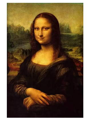
In the eyes of the machine, the human face looks like this:

You read it right, the image is stored in the machine but it's a binary string of 0s and 1s! More precisely, the machine sees the color value of each point on the image, so for a machine, an image is an array of numbers. Imagine if I read the color values ​​of each point to you. Can you tell me if there are any faces and faces on this image? Obviously, this is not an easy problem to solve.
If a mobile phone can't find our face in a selfie, it's like a blinding makeup artist, unable to show our best side; if the attendance machine can't see our face through the camera, then our laugh It's just a matter of affection. It's impossible to identify who we are. Face detection builds a bridge between the machine and us, enabling it to know our identity (face recognition), read our expressions (expression recognition), laugh with us (face animation), and Interaction together (human-computer interaction).
The start and basic flow of face detection
Specifically, the task of face detection is to determine whether there is a face on a given image. If the face exists, it gives the position and size of all faces. Due to the importance of face detection in practical applications, people began to research as early as the 1970s. However, due to the backward technical conditions and limited demand, until the 1990s, face detection technology began. To accelerate the pace of development, in the last decade before the arrival of the new century, a large number of researches on face detection have emerged. Many face detectors designed during this period have already had the shadow of modern face detection technology. For example, The design of the deformable template (the face is divided into a plurality of interconnected partial blocks according to the features and contours), the introduction of a neural network (as a classification model for judging whether the input is a face), or the like. These early work focuses on detecting the frontal face, analyzing the image based on simple underlying features such as the edge of the object, the gray value of the image, etc., and combining the prior knowledge on the human face to design the model and algorithm (such as features, Skin color) and began to introduce some existing pattern recognition methods.
Although early research work on face detection is far from the requirements of practical application, the process of detection has no essential difference with modern face detection methods. Given an input image, to complete the task of face detection, we usually divide it into three steps:
1. Select a (rectangular) area on the image as a viewing window;
2. Extract some features in the selected window to describe the image area it contains;
3. According to the feature description to determine whether the window is exactly framed by a human face.
The process of detecting faces is to continuously perform the above three steps until all windows that need to be observed are traversed. If all the windows are judged not to contain faces, then it is considered that there is no face on the given image, otherwise the position and size of the faces are given based on the window determined to contain faces.
So how do you choose the window we want to observe? The so-called seeing is true, to determine whether a certain position on the image is a face, it must be observed after this position is known, therefore, the selected window should cover all positions on the image. Obviously, the most direct way is to let the viewing window slide from left to right, from top to bottom, and from the top-left corner of the image to the bottom-right corner of the image—this is the so-called sliding window paradigm. You can It is thought of as the process by which Holmes (detector) looks at each corner (sliding) of the scene (input image) of the scene with a magnifying glass (observation window).
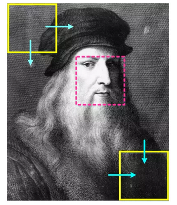
Do not look at this kind of window scanning method on the image is very simple and crude, it is indeed an effective and reliable window selection method, so that until today, the sliding window paradigm is still used by many face detection methods, rather than Sliding window detection methods are still essentially free from the intensive scanning of images.
Another important question for the observation window is: How large should the window be? We think that a window is a face window if and only if it exactly framed a face, that is, the size of the window is the same as the size of the face, and the window basically conforms to the outline of the face.
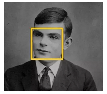
Then the question is, even if it is the same image, the size of the face is not only not fixed, but also can be arbitrary, so how can we make the observation window adapt to different sizes of human faces? One approach is of course to use multiple windows of different sizes to scan the images separately, but this approach is not efficient. From a different point of view, it is also possible to scale the image to different sizes and then use the same size window to scan - this is the so-called way of constructing an image pyramid. The name of the image pyramid is very vivid. The images that are scaled to different sizes are stacked in order from the largest to the smallest, just in the shape of a pyramid.
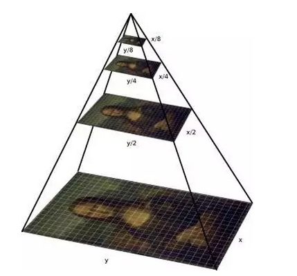
By constructing an image pyramid and allowing the fit of the window and face to move within a small range, we can detect faces of different locations and sizes. In addition, it should be mentioned that for human faces, we usually only use a square observation window, so we do not need to consider the aspect ratio of the window.
Having chosen the window, we began to observe the image area in the window, the purpose is to collect evidence - the truth is only one, we have to rely on evidence to discover the truth! In the process of processing images, this link of collecting evidence is called feature extraction. The feature is our description of the image content. Since the machine sees only a bunch of values ​​and can only deal with values, the feature extracted from the image is represented by a vector, called a feature vector. Each dimension is a value. The value is based on the input. The (image area) is obtained by some calculations (observation), such as summation, subtraction, comparison of sizes, and the like. In a word, the feature extraction process is the process of transforming the original input data (matrix composed of the color values ​​of the image regions) into the corresponding feature vectors. The feature vectors are the evidence we use to analyze and find the truth.
After feature extraction, it is time for a decision: determine if the current window contains exactly one face. We divide all the windows into two categories. One is a window that exactly contains the face, called the face window. The rest is classified as the second type. We call it the non-human face window, and the final decision process is A process of classifying the current viewing window. Because our evidence is eigenvectors of numerical values, we are looking for the truth through computational mathematical models. The mathematical model used to deal with classification problems is commonly called a classifier. The classifier takes the feature vector as input. Through a series of mathematical calculations, using categories as output - each category will correspond to a numeric code, called the tag corresponding to this category. For example, the face window is encoded as 1 instead of the face window. The class code is -1; the classifier is a function that transforms feature vectors into class labels.
Consider one of the simplest classifiers: add the values ​​in each dimension of a feature vector, and if the sum exceeds a certain value, output the category label of the face window, otherwise, output the category label of the non-face window -1. . Remember the feature vector is

The classifier is function f(x), then there are:

Here t is the aforementioned "some value", which determines the output of the classifier under a given feature vector, which we call the classifier's parameters. Different types and types of classifiers have different parameters. A classifier may have one or more parameters. Parameters or their values ​​may be different for different classifiers. After selecting a classifier, the next question is: how to set the parameters? Specific to the situation we are considering, is: how to choose the value of t?
To make a choice, there must be a goal. In the classification problem, the goal is of course to classify it as accurately as possible, that is, the classification accuracy is as high as possible. However, although we are very clear about the goal, we still cannot give an optimal parameter value, because we do not use the binary language system used by the machine, and we do not know what is best for the machine. So we have only one choice: tell our machine our goal, explain it to some examples, and let the machine learn this parameter by itself. Finally we design an exam for the machine and test whether it meets our requirements. We select some examples of face and non-face windows from some images, annotate them with corresponding category labels, and then divide these samples into two sets. One set is used as a training for classifier learning. Set, another set as a test set that ultimately examines the capabilities of the classifier, and we set a goal: We hope that the accuracy of the classification can be more than 80%.
At the beginning of the learning process, we first set an initial value for the parameters of the classifier, and then let the classifier continuously adjust the value of its own parameter to narrow it by training the sample with the answer (category tag). The difference between actual classification accuracy and target accuracy. When the classifier has reached a pre-set goal or other conditions that stop learning - the time for the final exam will not be postponed because you did not learn it well, or the classifier feels that it has no way to re-adjust it, and the learning process stops After this, we can examine the accuracy of the classifier on the test set as a basis for our evaluation of the classifier. In this process, the way in which the classifier adjusts its own parameters is related to the type of the classifier, the set target, etc. Since this part is beyond the scope of this article, it does not affect the reader's understanding of the face detection method. , so no longer talk about it.
After determining the strategy of choosing a window, designing a way to extract features, and learning a classifier for face and non-face windows, we have obtained all the key elements needed to build a face detection system— - There are some small links that are not as important as they are. This is omitted for the time being.
Since the sliding window method is used to discriminate face and non-human face windows at each position on images of different sizes, for a single input image with a size of 480320, the total number of windows is already as high as several hundred thousand. For such a huge input scale, if the speed of feature extraction and classification for a single window is not fast enough, it will easily cause a huge time overhead for the entire detection process, and it is really because of this, the face detector processing speed designed earlier It's very slow. An image can take a few seconds to complete. The video playback speed is usually 25 frames per second, which poses a serious obstacle to the application of face detection to real-world applications.
Breakthrough in Face Detection Technology: VJ Face Detector and Its Development
The breakthrough in face detection technology took place in 2001. Two prominent scientific researchers, Paul Viola and Michael Jones, designed a fast and accurate face detector: with the same or even better accuracy, the speed increases. Hundreds and hundreds of times - at the time of the hardware conditions to achieve 15 images per second speed, has been close to real-time speed 25fps (25 frames per second). This is not only a milestone in the development of face detection technology, but also marks that the research results in the field of computer vision have begun to put into practical application. To commemorate this work, people named the face detector with two scientific researchers named Viola-Jones face detector or simply VJ face detector.
VJ face detection algorithm can achieve success, greatly improve the speed of face detection, which has three key elements: the rapid calculation of features - the integral diagram, effective classifier learning methods - AdaBoost, and efficient classification strategy - Design of cascaded structures. The VJ face detector uses the Haar feature to describe each window. The so-called Haar feature is actually taking a small rectangular block at a certain position in the window, and then dividing the rectangular small block into black and white parts and respectively The sum of the gray values ​​of the pixels covered by the two parts (each point on the image is called a pixel) is summed, and the sum of the gray values ​​of the black part pixels is subtracted from the sum of the gray values ​​of the white part pixels. The value of a Haar feature.

The Haar feature reflects the relative brightness and darkness between local regions. It can provide effective information for distinguishing between human face and non-human face. For example, the eye region is darker than the surrounding skin region. This feature can be expressed through the Haar feature. However, since the sum of the gray values ​​of multiple pixel points in the local area needs to be calculated each time the Haar feature is extracted, it is not fast in speed. For this reason, the VJ face detector introduces an integral graph to accelerate the extraction of Haar features.
The integral graph is a graph that is as large as the input image, but at each point it is no longer the grayscale value that holds this point, but instead stores the grey point from the upper left corner of the image to all points in the rectangular area defined by that point. The sum of the degrees.
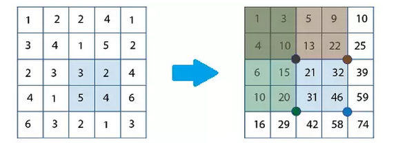
The advantages of the integral graph are two aspects. On the one hand, it makes the sum of the gray values ​​of the pixels in the local area only need to be added and subtracted 4 times each time, regardless of the size of the local area; on the other hand, it avoids Repeated summation at the same pixel point is only calculated once at the very beginning—adjacent windows have a large overlap, the corresponding Haar features will also overlap, if you recalculate the gray value of the pixel each time And, the calculation of overlapping parts is repeated. The integration graph greatly accelerates the extraction of Haar features and takes the first step toward a fast detector.
In addition to feature extraction, the speed of the classification process is also critical for the speed of detection. The speed of classification depends on the complexity of the classifier, that is, the complexity of the calculation process from the feature vector to the class label. Complex classifiers often have stronger classification ability and can obtain better classification accuracy, but the calculation cost is higher when classifying, while a simple classifier has low computational cost, but the classification accuracy is also low. Is there any way to balance the cost of calculation and classification accuracy? Of course, this is the AdaBoost method. We hope that the computational cost is small, so we only use a simple classifier, but we also hope that the classification accuracy is high, so we combine multiple simple classifiers—weak and strong, combining multiple weak classifiers into one strong classifier. This is the core idea of ​​the AdaBoost method. Classifiers are learned by the AdaBoost method, which achieves the same accuracy of classification with less computational cost.
The underlying reason for the slow speed of face detection is that the input scale is too large, and it is often necessary to handle tens of millions of windows. If such an input scale is unavoidable, then is it possible to reduce the input size as quickly as possible during processing? What? If you can quickly eliminate most of the windows by a rough observation, leaving only a small part of the window to be carefully identified, the overall time overhead will be greatly reduced. Starting from this idea, VJ face detector uses a cascade structure to gradually reduce the input size.

Specifically, the VJ Face Detector cascades multiple classifiers, and the complexity and computational cost of the classifier gradually increases from the point of departure. For a given window, it is ranked first and most A simple classifier categorizes the window. If the window is classified as a non-face window, it is not sent to the next classifier for classification and is directly excluded. Otherwise, it is sent to the next classifier to continue the discrimination until it Be excluded, or be divided into face windows by all classifiers. The benefits of this design are obvious. Every time a classifier is passed, the window to be discriminated by the next classifier will be reduced, making it possible to eliminate most non-face windows with only a very small computational cost. From another perspective, this actually adjusts the classifier's complexity dynamically based on the difficulty of a window classification, which is obviously more efficient than using the same classifier for all windows.
The great success of the VJ face detector through the integration graph, AdaBoost method, and cascade structure has had a profound impact on the subsequent research on face detection technology. A large number of researchers have begun to make improvements based on the VJ face detector. It also covers the three key elements of the VJ face detector.
Improvements and changes in characteristics
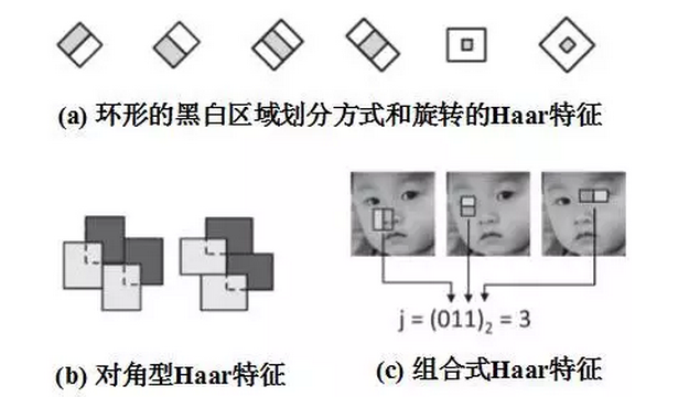
Although the Haar feature has been able to portray some features of the human face, the five Haar features used by the VJ face detector are still too simple compared to the complex face change modes. Light considers changes in posture. Faces may be oblique (in-plane rotation), or upside-down (out-of-plane rotation), and the same Haar feature may be very different in faces of different poses. Large, but at the same time may be more similar to features on non-face areas, which can easily cause misjudgments when categorized. So people began to extend the Haar feature so that it can portray a richer change pattern:
1. The circular black and white area dividing mode, not just up and down or left and right;
2. The characteristics of the rotating Haar, that is to say, the local small piece of the original Haar feature is rotated clockwise or counterclockwise by 45 degrees;
3. Separate Haar features that allow a Haar feature to be calculated from multiple black and white areas that are separated from one another, without requiring that the black and white areas must be in a rectangular block;
4. Diagonal Haar features;
5. Combining Haar features, ie combining multiple Haar features and binary coding;
6. Locally combined binary features, that is, locally combining specific Haar features with a certain structure and binary coding;
7. Weighted multi-channel Haar feature, that is, a Haar feature no longer contains only black and white blocks, but allows a variety of different shapes and different color blocks, where different colors correspond to different weights, representing pixel points The proportion after the summation - originally only two kinds of 1 and -1, multi-channel means that the summation at the pixel point is not only calculated on the grayscale channel, but is also calculated on other channels ( For example, three color channels of RGB; in fact, any graph calculated based on the original image and the same size as the original image can be a channel of the image).
These extensions greatly enhance the expressiveness of Haar features, making the distinction between face windows and non-human face windows better, thereby improving the accuracy of the classification.
In addition to directly improving Haar features, people are also designing and experimenting with other features. The Haar feature is essentially a linear combination of pixel values ​​in a local area. The corresponding more general form is a coefficient that does not specify a linear combination. The allowed coefficient is an arbitrary real number. This is called a linear feature—the combination here. Coefficients can be learned based on training examples, similar to the process of learning classifier parameters. The sparse granularity feature is also a feature based on linear combination. Unlike the linear feature, the sparse granularity feature is different scale (100100 image is enlarged to 200200, it is different from the original image size is 200200 The local areas of the scale, location, and size are combined, whereas the linear features only combine pixel values ​​within the same local area.
The LBP feature is a binary coding feature, which is directly calculated based on the pixel gray value. The feature is that the relative size of the two values ​​is considered in coding, and coding is performed according to a certain spatial structure, and the local combined binary feature is used. It is designed under the inspiration of the LBP feature. From a computational point of view, extracting the LBP feature is faster than extracting the Haar feature, but the Haar feature is superior to the ability to discriminate between face and non-human face windows. The simplified SURF feature is a feature similar to the Haar feature, but it computes the gradient sum of the pixel points in the local area and considers the gradient direction during the summation (so-called gradient, the simplest case). It means that the difference between the pixel values ​​of two different positions on the same line is less than the horizontal coordinate of them; the SURF feature is more complicated than the Haar feature, so the calculation cost is higher, but because of its stronger expression ability, it can be reduced to a smaller number. The purpose features to achieve the same degree of differentiation, to a certain extent, make up for its lack of speed. The HOG feature is also a gradient-based feature that counts gradients in different directions within a local area and computes a gradient histogram to represent this area. The integral channel feature is similar to the multi-channel Haar feature, but the channel used is more diverse. The concept of the channel is extended to any image that is transformed from the original image and whose spatial structure corresponds to the original image. The characteristics of the aggregated channel further add downsampling operations to each channel based on the characteristics of the integrated channel, thereby realizing the aggregation of local area information.
In the course of exploration over the past decade or so, there are numerous features emerging. Here only some of the features that are representative and reflect people's thinking are selected as examples. All the features listed here have a common characteristic: they are hand-designed by scientific researchers based on their own experience. The design of these features reflects people's understanding and thinking of the problem. Although with the constant improvement, the characteristics of the design have been improved, but until now, people's exploration of the characteristics is far from over.
Classifiers and Improvements in Their Learning Methods
The strength of the classifier directly determines the level of classification accuracy, and the computational cost of the classification is a key factor affecting the detection speed. Therefore, another direction that people explore is the improvement of the classifier and its learning methods.
The AdaBoost method is used to construct strong classifiers from weak classifiers. This is a sequential execution process. In other words, once a weak classifier is selected, it must be part of a strong classifier. Do not allow estoppel. This is actually an assumption. Increasing the weak classifier will definitely make the classification of the strong classifier more accurate, but this assumption does not always hold. In fact, each time the choice of weak classifiers is only determined according to the circumstances at the time, and as the new weak classifiers are added, the overall choice is not necessarily optimal. Based on this idea, there is a FloatBoost method that allows backtracking. The FloatBoost method will also re-examine the original weak classifier while selecting the new weak classifier. If the classifier accuracy of the strong classifier is improved after removing a weak classifier, it indicates that the weak classifier brings Negative effects should be removed.
In the VJ face detector, multiple cascaded classifiers do not have a direct connection during the learning process. The correlation is only reflected in the training examples: the training examples of the classifier in the next stage must be preceded by Through the previous classifier. The independence of different classifiers in learning can bring about two disadvantages: one is that each classifier starts from scratch, cannot learn from the experience of previously learned classifiers, and the other is that each classifier is classified. You can only rely on yourself and cannot use information already obtained by other classifiers. For this reason, two improved schemes have emerged: the chained Boosting method and the nested Boosting method. Both schemes are considering classifiers that have been learned before when learning a new classifier. The difference is that the chained Boosting method directly accumulates the outputs of the preceding classifiers as a base score, and outputs the new classifiers. As an additional score, in other words, the former classifiers are actually a “prefix†of the new classifier. All classifiers are chained together in this way; nested Boosting method directly to the previous classifier. The output is used as a feature of the first weak classifier of the new classifier to form a nested relationship. Its characteristic is that only adjacent classifiers will influence each other. There is also a similar scheme to the nested Boosting method: feature inheritance, which is to associate different classifiers from the perspective of features rather than classifiers. Specifically, the new classifiers will inherit the previous class when learning. All features of the classifier learn weak classifiers based on these features, and then consider adding new weak classifiers on the basis. The characteristic of this solution is that it only introduces the mutual influence of classifier learning, and classifies The devices are still independent of each other.
Relevant tasks tend to promote each other and complement each other. One task that is closely related to face detection is feature point location: predicting the position of key points on the face. These key points can be the center of the eyes, the tip of the nose, and the corners of the mouth. Based on such an idea, Joint Cascade emerged in 2014 by alternately cascading the classifiers needed to detect faces and the regression of predicted feature points, and performing both face detection and feature point location tasks. The key to using feature point location to assist face detection lies in the introduction of shape indexing features. That is, features are not extracted in the entire window, but are extracted in a local area centered on each feature point. The advantage of this is that it improves The semantic consistency of features. Different facial features correspond to different feature point positions. Conversely, that is, the same position actually corresponds to different regions of the face, and features extracted in the same region actually represent different semantics. Simply put, it's matching noses and mouths. Using the shape index feature can be a good way to avoid this problem, thereby increasing the distinction between face and non-human face windows. For a given window, we do not know the position of the feature points, so we use an “average position†as the initial position, that is, the average of each point coordinate calculated based on the face sample set marked with the feature point coordinates. Values; Based on the average position, we extract features to predict the true position of each feature point, but one prediction is often inaccurate, as if we couldn't jump from the starting point to the end point directly when running, so we need to constantly base on the current Determine the location of the feature point to predict the new location and gradually move closer to its true location. This process naturally forms a cascade structure that can be coupled with a face detector to form a cascade of different models.
For each link in the classifier learning process, people have carried out meticulous and full exploration. In addition to the above-mentioned several directions, there are also problems in classifier classification threshold learning and speed of classifier learning. A lot of excellent research work. Most of the work on improving the classifier and its learning methods focuses on the Boosting method (AdaBoost method is an outstanding representative of the Boosting method) and the relatively simple classifier form. If a classifier with stronger classification ability can be introduced, It is believed that this will bring further performance improvements to the detector. This will be covered later in this article.
The evolution of cascade structure
The organizational structure of the classifier is also an important issue that people are concerned about, especially when faced with multi-pose face detection tasks. The face pose refers to the angle of the human face rotating in three-dimensional space around the three coordinate axes, and multi-pose face detection is to detect the face with rotation, whether it is oblique (rotate around the x axis) , reclining (rotating around the y-axis) or flanking (rotating around the z-axis). There are great differences in the appearance characteristics of human faces in different poses, which poses a great challenge to the detector. In order to solve this problem, a separate strategy is usually adopted, ie, the faces of different poses are separately The classifiers are trained and then combined to construct a multi-pose face detector.
The simplest multi-pose face detector is to organize the classifiers for different gesture faces using a side-by-side structure. Each of the parallel classifiers still uses the original cascade structure (we call this type of classifier In the process of detecting faces, if a window is divided into face windows by one of the cascaded classifiers, it is considered to be a face window, and only if each cascade classifier has its When it is judged as a non-face window, it is excluded. This kind of side-by-side organizational structure has two defects: First, it causes the detection time to grow exponentially because most windows are non-face windows. These windows need to be eliminated by each cascaded classifier. Second, it is easy. This leads to a reduction in the overall classification accuracy because the entire detector error window contains a window of error for all cascaded classifiers.
Someone has designed a pyramidal cascade structure. Each layer of the pyramid corresponds to a division of the face pose (rotation angle), and the partition from the top layer to the bottom layer is increasingly finer. Each classifier cascaded is only responsible for Distinguish between non-human faces and faces within a certain range of angles. For a window to be classified, it is classified from the top-most classifier and if it is divided into face windows, the first classifier sent to the next layer continues to classify if it is classified as non-classified. The face window is sent to the next classifier in the same layer to continue the classification. When all the classifiers on a certain layer classify it into non-face windows, it is confirmed as a non-human face window. Excluded. The pyramidal cascade structure can also be seen as a special parallel structure, except that each cascaded classifier has shared parts with each other, so the most direct benefit is that it reduces the amount of computation and the shared part. It only needs to be calculated once, while at the same time retaining the benefits of the divide-and-conquer strategy at the bottom level - the sub-problem is easier than the original problem, so it is easier to learn the classifier with higher classification accuracy.
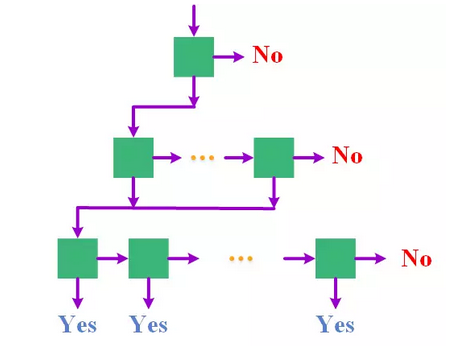
Another typical structure is a tree-like cascade structure. From the perspective of shape, it is the same as the pyramidal cascade structure. It is also the number of classifiers from top to bottom. The difference lies in the tree. In the cascade structure, there is no horizontal connection between the same layer classifiers, and only the vertical connection between the classifiers of adjacent layers, that is, one window is not classified by multiple classifiers on the same layer, but is directly sent to the same layer. The next layer is either excluded. The tree-like cascade structure further reduces the amount of computation needed to classify a window by introducing a branch-jump mechanism, but it also introduces new problems. Branch jumps are usually based on pose estimation (estimation of the range of rotation angles). The result is performed, and if the posture estimation error occurs, the face window of a certain gesture is sent to a classifier corresponding to another gesture face for classification, which easily leads to an incorrect classification. In order to alleviate this problem, there have been designs that allow multiple branches to jump at the same time, thereby reducing the risk of classification errors due to jump errors.
Divide-and-conquer strategy is the most basic strategy to deal with multi-pose face detection tasks, but it is not an easy task to balance speed and classification accuracy at the same time. The enhancement of classification ability will inevitably lead to increase of computational cost. Using smaller computational costs in exchange for higher classification accuracy is still a question that needs to be considered and explored.
Face detector competition
在ä¸æ–对人脸检测器进行改进的过程ä¸ï¼Œæœ‰ä¸€ä¸ªé—®é¢˜æ˜¯ä¸å®¹å¿½è§†çš„:如何科å¦åœ°æ¯”较两个人脸检测器的优劣?简å•åœ°è¯´ï¼Œå‡ºä¸€å¥—考题让所有的检测器进行一场考试,è°å¾—分高è°å°±æ›´å¥½ã€‚对于人脸检测器而言,所谓考题(测试集)就是一个图åƒé›†åˆï¼Œé€šå¸¸å…¶ä¸æ¯å¼ 图åƒä¸Šéƒ½åŒ…å«è‡³å°‘ä¸€å¼ äººè„¸ï¼Œå¹¶ä¸”è¿™äº›äººè„¸çš„ä½ç½®å’Œå¤§å°éƒ½å·²ç»æ ‡æ³¨å¥½ã€‚关于得分,需è¦è€ƒè™‘检测器两方é¢çš„表现,一是检测率,也å³å¯¹äººè„¸çš„å¬å›žçŽ‡ï¼Œæ£€æµ‹å‡ºæ¥çš„人脸å 总人脸的比例——测试集ä¸ä¸€å…±æ ‡æ³¨äº†100å¼ äººè„¸ï¼Œæ£€æµ‹å™¨æ£€æµ‹å‡ºå…¶ä¸70å¼ äººè„¸ï¼Œåˆ™æ£€æµ‹çŽ‡ä¸º70%;二是误检(也称为虚è¦ï¼‰æ•°ç›®ï¼Œå³æ£€æµ‹å™¨æ£€æµ‹å‡ºæ¥çš„人脸ä¸å‡ºçŽ°é”™è¯¯ï¼ˆå®žé™…上ä¸æ˜¯äººè„¸ï¼‰çš„数目——检测器一共检测出80å¼ äººè„¸ï¼Œç„¶è€Œå…¶ä¸æœ‰10个错误,åªæœ‰70个是真æ£çš„人脸,那么误检数目就是10ã€‚åœ¨è¿™ä¸¤ä¸ªæŒ‡æ ‡ä¸Šï¼Œæˆ‘ä»¬æ‰€å¸Œæœ›çš„æ€»æ˜¯æ£€æµ‹çŽ‡å°½å¯èƒ½é«˜ï¼Œè€Œè¯¯æ£€æ•°ç›®å°½å¯èƒ½å°‘ï¼Œä½†è¿™ä¸¤ä¸ªç›®æ ‡ä¹‹é—´ä¸€èˆ¬æ˜¯å˜åœ¨å†²çªçš„;在æžç«¯çš„æƒ…å†µä¸‹ï¼Œå¦‚æžœä¸€å¼ è„¸ä¹Ÿæ²¡æœ‰æ£€æµ‹å‡ºæ¥ï¼Œé‚£ä¹ˆè¯¯æ£€æ•°ç›®ä¸º0,但是检测率也为0,而如果把所有的窗å£éƒ½åˆ¤åˆ«ä¸ºäººè„¸çª—å£ï¼Œé‚£ä¹ˆæ£€æµ‹çŽ‡ä¸º100%ï¼Œè€Œè¯¯æ£€æ•°ç›®ä¹Ÿè¾¾åˆ°äº†æœ€å¤§ã€‚åœ¨æ¯”è¾ƒä¸¤ä¸ªæ£€æµ‹å™¨çš„æ—¶å€™ï¼Œæˆ‘ä»¬é€šå¸¸å›ºå®šä¸€ä¸ªæŒ‡æ ‡ï¼Œç„¶åŽå¯¹æ¯”å¦ä¸€ä¸ªæŒ‡æ ‡ï¼Œè¦ä¹ˆçœ‹ç›¸åŒè¯¯æ£€æ•°ç›®æ—¶è°çš„检测率高,è¦ä¹ˆçœ‹ç›¸åŒæ£€æµ‹çŽ‡æ—¶è°çš„误检少。
对于æ¯ä¸€ä¸ªæ£€æµ‹å‡ºçš„人脸,检测器都会给出这个检测结果的得分(或者说信度),那么如果人为地引入一个阈值æ¥å¯¹æ£€æµ‹ç»“果进行ç›é€‰ï¼ˆåªä¿ç•™å¾—分大于阈值得检测结果),那么éšç€è¿™ä¸ªé˜ˆå€¼çš„å˜åŒ–,最终得检测结果也会ä¸åŒï¼Œå› 而其对应得检测率和误检数目通常也会ä¸åŒã€‚通过å˜æ¢é˜ˆå€¼ï¼Œæˆ‘们就能够得到多组检测率和误检数目的值,由æ¤æˆ‘们å¯ä»¥åœ¨å¹³é¢ç›´è§’åæ ‡ç³»ä¸ç”»å‡ºä¸€æ¡æ›²çº¿æ¥ï¼šä»¥xåæ ‡è¡¨ç¤ºè¯¯æ£€æ•°ç›®ï¼Œä»¥yåæ ‡è¡¨ç¤ºæ£€æµ‹çŽ‡ï¼Œè¿™æ ·ç”»å‡ºæ¥çš„曲线称之为ROC曲线(ä¸åŒåœ°æ–¹ä¸æ–‡è¯‘法ä¸ä¸€ï¼Œå¦‚接收机曲线ã€æŽ¥æ”¶è€…æ“作特å¾æ›²çº¿ç‰ï¼Œè¿™é‡Œç›´æŽ¥é‡‡ç”¨è‹±æ–‡ç®€å†™ï¼‰ã€‚ROC曲线æ供了一ç§éžå¸¸ç›´è§‚的比较ä¸åŒäººè„¸æ£€æµ‹å™¨çš„æ–¹å¼ï¼Œå¾—到了广泛的使用。
评测人脸检测器时还有一个é‡è¦çš„é—®é¢˜ï¼šæ€Žä¹ˆæ ¹æ®å¯¹äººè„¸çš„æ ‡æ³¨å’Œæ£€æµ‹ç»“æžœæ¥åˆ¤æ–æŸå¼ 人脸是å¦è¢«æ£€æµ‹åˆ°äº†ï¼Ÿä¸€èˆ¬æ¥è¯´ï¼Œæ£€æµ‹å™¨ç»™å‡ºçš„检测框(å³äººè„¸çª—å£ï¼‰ä¸ä¼šå’Œæ ‡æ³¨çš„äººè„¸è¾¹æ¡†å®Œå…¨ä¸€è‡´ï¼Œè€Œä¸”å¯¹äººè„¸çš„æ ‡æ³¨ä¹Ÿä¸ä¸€å®šæ˜¯çŸ©å½¢ï¼Œä¾‹å¦‚还å¯èƒ½æ˜¯æ¤åœ†å½¢ï¼›å› æ¤å½“ç»™å®šäº†ä¸€ä¸ªæ£€æµ‹æ¡†å’Œä¸€ä¸ªæ ‡æ³¨æ¡†æ—¶ï¼Œæˆ‘ä»¬è¿˜éœ€è¦ä¸€ä¸ªæŒ‡æ ‡æ¥ç•Œå®šæ£€æµ‹æ¡†æ˜¯å¦å’Œæ ‡æ³¨æ¡†ç›¸åŒ¹é…ï¼Œè¿™ä¸ªæŒ‡æ ‡å°±æ˜¯äº¤å¹¶æ¯”ï¼šä¸¤è€…äº¤é›†ï¼ˆé‡å 部分)所覆盖的é¢ç§¯å 两者并集所覆盖é¢ç§¯çš„æ¯”ä¾‹ï¼Œä¸€èˆ¬æƒ…å†µä¸‹ï¼Œå½“æ£€æµ‹æ¡†å’Œæ ‡æ³¨æ¡†çš„äº¤å¹¶æ¯”å¤§äºŽ0.5时,我们认为这个检测框是一个æ£ç¡®æ£€æµ‹çš„人脸。
在早期的人脸检测工作ä¸ï¼Œä¸€èˆ¬é‡‡ç”¨MIT-CMU人脸检测数æ®é›†ä½œä¸ºäººè„¸æ£€æµ‹å™¨çš„测试集,æ¥æ¯”较ä¸åŒçš„检测器。这个测试集åªåŒ…å«å‡ ç™¾å¼ å¸¦æœ‰äººè„¸çš„å›¾åƒï¼Œå¹¶ä¸”人脸主è¦æ˜¯æ¸…晰且ä¸å¸¦é®æŒ¡çš„æ£é¢äººè„¸ï¼Œå› 而是一个相对简å•çš„æµ‹è¯•é›†ï¼ŒçŽ°åœ¨å‡ ä¹Žå·²ç»ä¸å†ä½¿ç”¨ã€‚在2010年,美国麻çœå¤§å¦çš„一个实验室推出了一个新的人脸检测评测数æ®é›†ï¼šFDDB,这个集åˆå…±åŒ…å«2845å¼ å¸¦æœ‰äººè„¸çš„äº’è”网新闻图åƒï¼Œä¸€å…±æ ‡æ³¨äº†5171å¼ äººè„¸ï¼Œå…¶ä¸çš„人脸在姿æ€ã€è¡¨æƒ…ã€å…‰ç…§ã€æ¸…晰度ã€åˆ†è¾¨çŽ‡ã€é®æŒ¡ç¨‹åº¦ç‰å„个方é¢éƒ½å˜åœ¨éžå¸¸å¤§çš„å¤šæ ·æ€§ï¼Œè´´è¿‘çœŸå®žçš„åº”ç”¨åœºæ™¯ï¼Œå› è€Œæ˜¯ä¸€ä¸ªéžå¸¸å…·æœ‰æŒ‘战性的测试集。FDDB的推出激å‘äººä»¬åœ¨äººè„¸æ£€æµ‹ä»»åŠ¡ä¸Šçš„ç ”ç©¶çƒæƒ…,æžå¤§åœ°ä¿ƒè¿›äº†äººè„¸æ£€æµ‹æŠ€æœ¯çš„å‘展,在æ¤åŽçš„å‡ å¹´é—´ï¼Œæ–°çš„äººè„¸æ£€æµ‹æ–¹æ³•ä¸æ–涌现,检测器在FDDB上的表现稳æ¥æ高。从100个误检时的检测率æ¥çœ‹ï¼Œä»Žæœ€åˆVJ人脸检测器的30%,å‘展到现在已ç»è¶…过了90%——这æ„味ç€æ£€æµ‹å™¨æ¯æ£€æµ‹å‡º50å¼ äººè„¸æ‰ä¼šäº§ç”Ÿä¸€ä¸ªè¯¯æ£€ï¼Œè¿™å…¶ä¸çš„è¿›æ¥æ˜¯éžå¸¸æƒŠäººçš„,而检测器之间的比拼还在继ç»ã€‚
雷锋网注:本文由作者å‘布于深度å¦ä¹ å¤§è®²å ‚ï¼Œè½¬è½½è¯·è”系授æƒå¹¶ä¿ç•™å‡ºå¤„和作者,ä¸å¾—åˆ å‡å†…容。
LiFePO4 Battery Pack refers to a battery pack that uses lithium iron phosphate (LiFePO4) as the positive electrode material, which is a common lithium-ion battery. LiFePO4 battery has been widely concerned and applied due to its advantages of high safety, long life, high energy density, and environmental protection.
Main effect:
Energy storage: The main function of the LiFePO4 Battery Pack is to store energy and store electrical energy so as to supply electricity to electrical equipment when needed. It can store electricity from solar panels or other power sources, and then supply power at night or when solar radiation is low.
Smooth power output: LiFePO4 battery has good power characteristics, can output power smoothly, and maintain a stable power supply. It can adjust and supplement power fluctuations to ensure the continuity and stability of the power supply.
Provide backup power: LiFePO4 Battery Pack can be used as a backup power source for power outages or emergencies, providing continuous power to critical equipment.
Differences from Solar Battery Pack:
Solar Battery Pack is a more general concept that refers to the overall unit formed by combining multiple solar battery cells. This battery pack can utilize different types of battery technologies, including lithium-ion batteries, lead-acid batteries, and more.
The LiFePO4 Battery Pack is a specific type of Solar Battery Pack, which refers to a solution that uses a lithium iron phosphate battery as a battery pack. Therefore, LiFePO4 Battery Pack is a subset of the Solar Battery Pack.
In general, LiFePO4 Battery Pack is a specific type of solar battery pack, which uses lithium iron phosphate lithium battery, which has the advantages of high safety and long life and is suitable for energy storage applications of solar power generation. The Solar Battery Pack is a broader concept, including all battery packs used to store solar energy or other energy, of which the LiFePO4 Battery Pack is just one of the implementations.
48v lifepo4 battery pack, lithium iron phosphate battery pack, lifepo4 battery pack 12v, custom lifepo4 battery packs, lifepo4 battery kit
Ningbo Autrends International Trade Co., Ltd. , https://www.china-energystorage.com