When it comes to machine learning, many people would recommend Stanford CSS 229. This article systematically organizes the course. Including supervised learning, unsupervised learning and deep learning. It can be described as a "handheld memo" for learning ML.
Stanford CS229—Machine Learning:
Supervised learning
Unsupervised learning
Deep learning
Machine Learning Memo-Supervised Learning
Introduction to Supervised Learning
Given a set of data points {x(1),...,x(m)} associated with the output {y(1),...,y(m)}, we hope to construct a The classifier that predicts the y value.
Forecast types-the table below summarizes the different types of forecasting models

Model type-the table below summarizes the different models

Symbols and concepts
Hypothesis-remember a hypothesis as hθ, and it is a model of our choice. Given a set of input data x(i), the model predictive output is hθ(x(i)).
Loss function—a loss function can be expressed as L:(z,y)∈R×Y⟼L(z,y)∈R, which takes the predicted value z corresponding to the actual data value y as input, and outputs between them The difference. Common loss functions are summarized as follows:
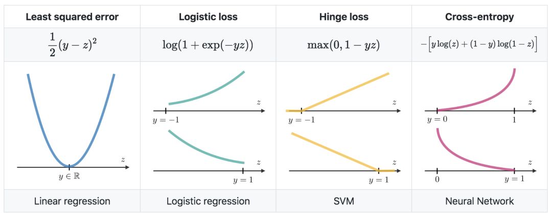
Cost function—The cost function J is usually used to evaluate the performance of the model. The loss function L is defined as follows:

Gradient descent—if the learning rate is expressed as α ∈ R, the update rule of gradient descent is defined by the learning rate and cost function J, which can be expressed as the following formula:
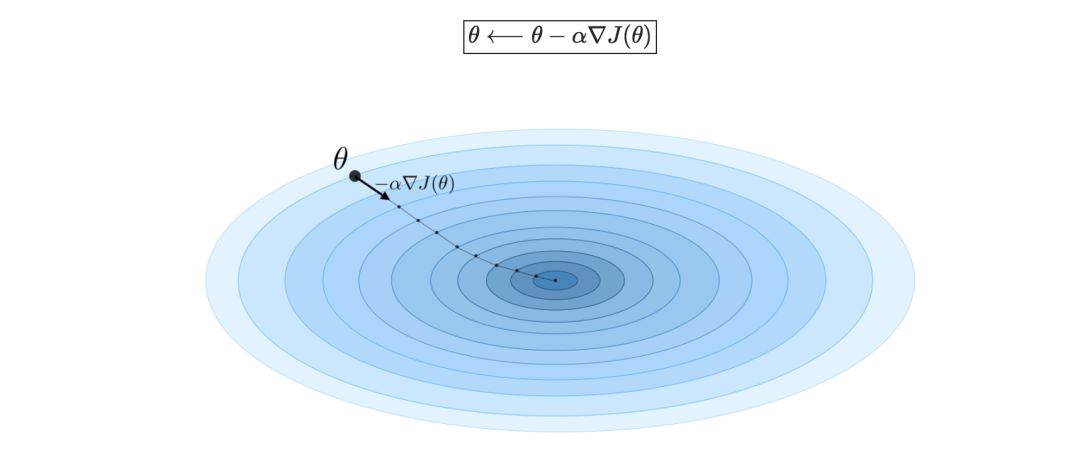
Stochastic gradient descent (SGD) is to update the parameters according to each training sample, and the batch gradient descent method is to update a batch of training samples
Likelihood—The likelihood of a model (given the parameter L(θ)) is to find the optimal parameter θ by maximizing it. In the actual process, we generally use the log likelihood ℓ(θ)=log(L(θ)), because the optimization operation is easier. It can be expressed as follows:

Newton iteration method-is a numerical method used to find a θ such that ℓ'(θ)=0 holds true. The update rules are as follows:

Linear model
Linear regression
We assume y|x; θ∼N(μ,σ2).
Normal Equation—Mark X as a matrix. The value of θ that minimizes the cost function is a closed solution:

Least Mean Square Algorithm (LMS)—denote α as the learning rate. The update rule of the LMS algorithm (also called Widrow-Hoff learning rule) of a training set containing m data points is as follows:

Locally Weighted Regression (LWR)—It is a variant of linear regression, which weights the cost function of each training sample as w(i)(x), which can be defined by the parameter τ∈R as:

Classification and logistic regression
Sigmoid function—S-type function, can be defined as:

Logistic regression-generally used to deal with two classification problems. Assuming y|x;θ∼Bernoulli(ϕ), it can have the following form:

Softmax regression-is a generalization of logistic regression, generally used to deal with multi-classification problems, which can be expressed as:

Generalized linear model
Exponential family—If a type of distribution can be represented by a natural parameter, then this type of distribution can be called an exponential family, also known as a regular parameter or link function, as shown below:

The following table shows some common exponential distributions:

Assumptions of the generalized linear model—The generalized linear model aims to predict a random variable y as a function of x∈Rn+1, and is based on the following three assumptions:

Support Vector Machines
In layman's terms, the support vector machine is to find a hyperplane and segment the samples.
Optimal edge classifier—denoted by h, which can be defined as:

Among them, (w,b)∈Rn×R is the solution of the following optimal problem:
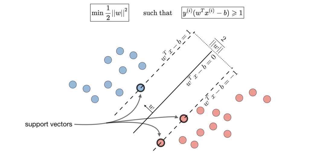
Hinge loss-used for SVM settings, defined as follows:

Kernel—Given a feature map ϕ, the kernel can be expressed as:

In practical problems, Gaussian kernels are more commonly used.
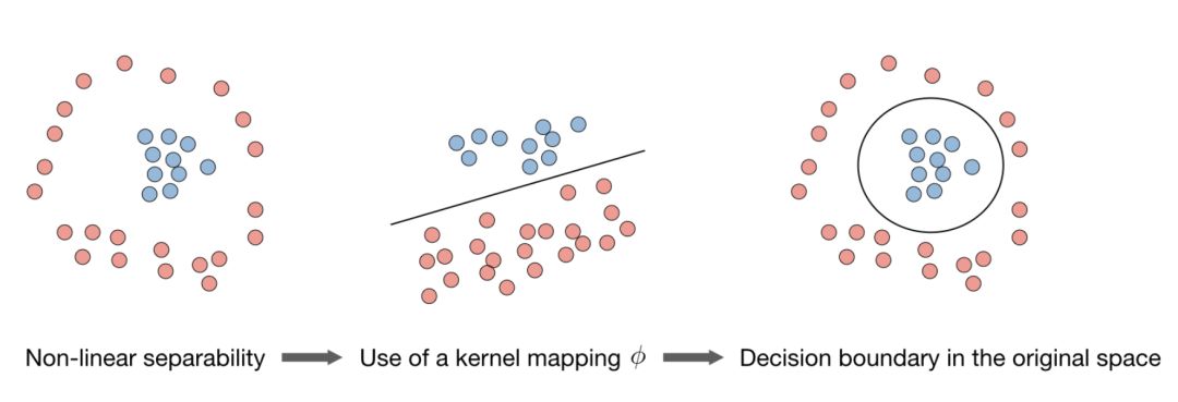
We generally don’t need to know the explicit mapping of XX, we only need to know the value of K(x,z)
Lagrange—we define Lagrange L(w,b) as:

Generative learning
The generative model first tries to understand how the data is generated by estimating P(x|y), and then we can use Bayes' rule to estimate P(y|x).
Gaussian Discriminant Analysis
Setting—Gauss discriminant analysis assumes that y, x|y=0 and x|y=1 exist, satisfying:

Estimates—The following table summarizes the estimates when maximizing likelihood:

Naive Bayes
Assumptions-the naive Bayes model assumes that the characteristics of each data point are independent:

Solution—When k∈{0,1},l∈[[1,L]], maximizing the log likelihood gives the following solution:

Tree-based method and integrated method
It can be used for regression and classification methods.
Decision tree-classification and regression tree (CART), very interpretable characteristics.
Boosting—The idea is to combine multiple weak learners to form a stronger learner.
Random Forest—Bootstrap is used on the samples and the features used. Unlike decision trees, its interpretability is weak.
Other non-parametric methods
KNN-k nearest neighbors, the response of a data point is determined by the nature of its k "neighbors".
Learning Theory
Union Bound—Let A1,...,Ak be k events, then:

Hoeffding inequality-describes the difference between the true probability of an event and the frequency observed in the Bernoulli test with different m.

Training error—given a classifier h, we define the training error as errorˆϵ(h), also known as empirical risk or empirical error, as shown below:

Probably Approximately Correct-PAC, is a framework under which many results about learning theories have been proven, and there are the following set of hypotheses:
The training and test sets follow the same distribution
Training samples are drawn independently
In addition to the above learning theories, there are concepts such as Shattering, upper limit theorem, VC dimension, Theorem (Vapnik), etc. If readers are interested, you can enter the original text from the link at the end of the article for further understanding.
Machine Learning Memo-Unsupervised Learning
Introduction to unsupervised learning
Unsupervised learning aims to discover patterns in unlabeled data.
Jensen's inequality—let f be a convex function and X be a random variable. There will be the following inequalities:

Clustering
Maximum Expectation Algorithm (EM)
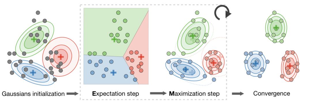
Hidden variable—refers to the hidden/unobserved variable that makes the estimation problem difficult to solve, usually expressed as z. The following table is the commonly used settings involving hidden variables:

Algorithm—EM algorithm provides an effective method for estimating the parameter θ through MLE by repeatedly constructing the lower bound of the likelihood (E-step) and optimizing the lower bound (M-step), as follows:
k-means clustering
Let c(i) be the class of data point i, and μj be the center of class j.
Algorithm—After randomly initializing the cluster centroids μ1, μ2,..., μk∈Rn, the k-means algorithm repeats the following steps until convergence:
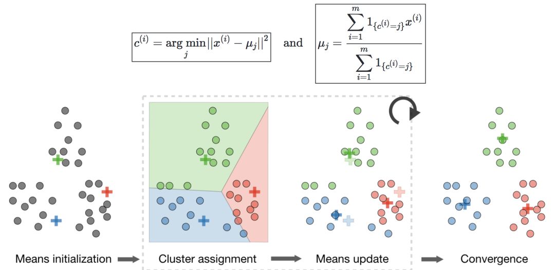
Distortion function (distortion function)—In order to see whether the algorithm has converged, define the following distortion function:

Hierarchical clustering
Algorithm—It is a clustering algorithm that uses an aggregation and hierarchical method to construct nested clusters in a continuous manner.
Type—In order to optimize different objective functions, there are different types of hierarchical clustering algorithms, as shown in the following table:

Cluster evaluation index
In an unsupervised learning environment, it is usually difficult to evaluate the performance of a model because there is no ground-truth label like in a supervised learning environment.
Contour coefficient-let a be the average of the distance between a sample and other points in the same class, and b be the average of the distance between a sample and all points in its nearest class. The contour coefficient of a sample can be defined as:

Calinski-Harabaz index—denote k as the number of classes, and XX and XX are the dispersion matrices of the inter-class and intra-class matrices, respectively, expressed as:

The Calinski-Harabaz index s(k) shows how well the clustering model defines clusters. The higher the score, the denser the clusters and the better the separation. It is defined as follows:

Dimensionality reduction
Principal component analysis
Principal component analysis is a statistical method. Transform a group of potentially correlated variables into a group of linearly uncorrelated variables through orthogonal transformation, and this group of variables after conversion is called principal component.
Eigenvalue, eigenvector—given a matrix A∈Rn×n, if there is a vector z∈Rn∖{0}, then λ is called the eigenvalue of A, and z is called the eigenvector:

Spectral theorem—let A ∈ Rn×n. If A is symmetric, then A can be diagonalized by the actual orthogonal matrix U∈Rn×n. Remember Λ=diag(λ1,...,λn), we have:

Algorithm-Principal Component Analysis (PCA) process is a dimensionality reduction technique, by maximizing the variance of the data, projecting the data on the k dimension, the method is as follows:
The first step: Standardize the data so that the mean is 0 and the standard deviation is 1.

Step 2: Calculation

The third step: Calculate the k orthogonal principal eigenvectors of Σ, that is, the orthogonal eigenvectors of the k largest eigenvalues.
Step 4: Project data on spanR(u1,...,uk).
This process maximizes the variance of all k-dimensional spaces.

Independent component analysis
This is a technique to find potential sources of generation.
Hypothesis-we assume that the data x is generated by the n-dimensional source vector s=(s1,...,sn) through the mixed and non-singular matrix A (where si is an independent random variable), then:

The goal is to find the mixing matrix W=A−1
Bell and Sejnowski's ICA algorithm—The algorithm finds the unmixing matrix W through the following steps:
Express the probability of x=As=W−1sx=As=W−1s as:

Let g be the sigmoid function. Given our training data {x(i),i∈[[1,m]]}, the log likelihood can be expressed as:

Therefore, the stochastic gradient ascent learning rule is that for each training sample x(i), we update W as follows:

Machine Learning Memo-Deep Learning
Neural Networks
A neural network is a type of model built with layers. Commonly used neural network types include convolutional neural networks and recurrent neural networks.
Structure-The description of the neural network architecture is shown in the following figure:

Let i be the i-th layer in the network and j be the j-th hidden unit in a layer. This is:

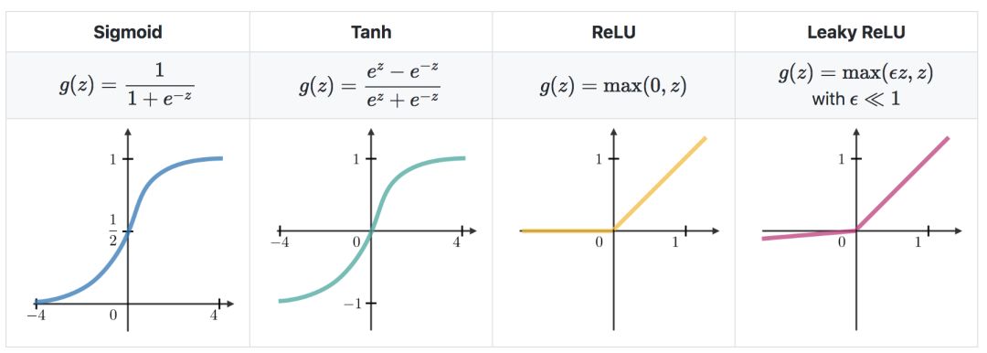
Activation function—Use the activation function at the end of the hidden unit to introduce nonlinear complexity to the model. The following are the most common ones:
Cross-entropy loss-In neural networks, cross-entropy loss L(z,y) is commonly used and is defined as follows:

Learning rate—usually recorded as α or η, it indicates at which step the weights are updated. This can be modified or changed adaptively. The most popular method currently is Adam, which is a method of adapting to the learning rate.
Backpropagation-is a method of updating the weight of a neural network by considering the actual output and expected output. The derivative of the weight w is calculated using the chain rule, and its form is as follows:

Therefore, the weights are updated as follows:

Update weights—In a neural network, the weights are updated as follows:
The first step: take a batch of training data;
Step 2: Perform forward propagation to obtain corresponding losses;
The third step: back propagation loss, get gradient;
Step 4: Use gradients to update the weights of the network.
Dropout-is a technique that prevents overfitting of training data by deleting units in a neural network.
Convolutional Neural Network
Hyperparameters—In the convolutional neural network, the following hyperparameters are corrected:

Types of layers—In a convolutional neural network, we may encounter the following types of layers:

Convolutional layer requirements-write W as the input size, F as the convolutional layer neuron size, P is the number of zero padding, then the number of neurons in a given volume (volumn) N is like this:

Batch normalization—remember γ, β as the mean and variance of the batch that we want to correct, then:

It is usually done before the fully connected/convolutional layer and the nonlinear layer, in order to increase the learning rate and reduce the strong dependence on initialization.
Recurrent neural network
Types of gates—The following are the different types of gates that exist in a typical recurrent neural network:

LSTM—This network is an RNN model that avoids the problem of vanishing gradients by adding "forget" gates.
Reinforcement learning and control
The goal of reinforcement learning is to let the agent learn how to evolve in the environment.
The Markov decision process—namely MDP, is a five-tuple (S,A,{Psa},γ,R), in which:
S is a set of states;
A is a set of behaviors;
{Psa} is the state transition rate of s∈S and a∈A;
γ∈[0,1] is the discount coefficient;
R:S×A⟶R or R:S⟶R is the reward function to be maximized by the algorithm
Bold: strategy—is a function π:S⟶A, which maps state to behavior.
Bold: Value Function—given a strategy π and state s, the value functionVπ can be defined
for:

Bellman equation—The optimal Bellman equation describes the value function of the optimal strategy π :
:

Value iterative algorithm-mainly divided into two steps:
Initialize value:

Iterate based on the previous value:

Maximum likelihood estimation-The maximum likelihood estimation of the state transition probability is as follows:

Q-Learning—is a model-free estimation of Q, the formula is as follows:

What suddenly appear into your mind when hear Mini Gaming PC? Is there quality heat-releasing fan and box design of Mini Gaming PC Build? Does it run stable and smoothly when handle heavier jobs, like Photoshop, Pr, engineering design and drawing, 3d Max, big games, etc. ? now we can be responsible to answer [ Yes". No matter cheap mini gaming pc or Mini Gaming PC Under $500, equips with quality fan to heat releasing. Therefore, no need to worry that again.
To processor, can do from intel celeron j4125, N5105 up to i3, i5 i7 10th 11th 12th with or without video graphics. To slots, same rich as traditional computer tower, like above 4 or 6 usb ports, 2 Rj45, VGA, PD, slot, etc.
You can also find Mini Gaming PC, j4125 Mini PC ,Custom All In One PC, windows 10 Education Laptop,Quad Core Processor Laptop, 15 Inch Gaming Laptop ,windows Yoga Laptop , 8 inch Android Tablet, etc.
If any other special requirements interest, you can also let us know, will try our best support you.
Meet your unique demand in this field is our mission, so just feel free contact us whenever you have different idea.
Mini Gaming PC Build,Cheap Mini Gaming PC,Mini Gaming PC Under $500,Mini Gaming Desktop
Henan Shuyi Electronics Co., Ltd. , https://www.shuyiaiopc.com